L1 tidbits |

Two mathematical tidbits that I came across recently, posted mainly for my own benefit.

1. L1 distance between probability density functions

If $X$ and $Y$ are two random variables with densities $f$ and $g$ , respectively, the density $f^*$ of the scaled variable $X^* = aX$ is

$f^*(x^*) = \frac{1}{a} f\Big(\frac{x^*}{a}\Big)\,,$

and similarly for $Y^*=aY$ , where $a>0$ . Using this transformation rule, we see that the $L_p$ distance between $f^*$ and $g^*$ satisfies

$\|f^*-g^*\|_p= a^{(1-p)/p}\|f-g\|_p\,.$

Setting $p=1$ , we get

$\|f^*-g^*\|_1= \|f-g\|_1\,.$

This latter result also holds for $m$ -dimensional vector random variables (for which the transformation rule is $f^*(x^*) = {1}/{a^m} f({x^*}/{a})$ ).

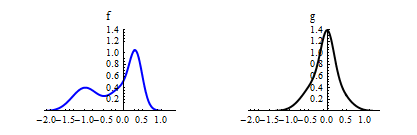
In their book on the $L_1$ approach to nonparametric density estimation, Luc Devroye and László Györfi prove a much more general version of this result, which includes as a special case the fact that $L_1$ distance between PDFs is invariant under continuous, strictly monotonic transformations of the coordinate axes. In the one-dimensional case, this means that one can have a visual idea about the $L_1$ distance between two PDFs by bringing the real line into a finite interval like $[-1,1]$ by a monotonic transformation.

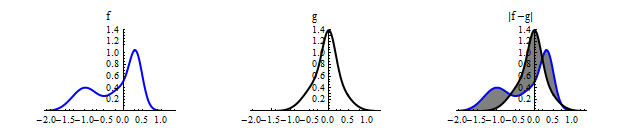
The figure below shows the transformed version of the PDFs above, via the transformations $X^* = \tanh{X}$ , $Y^* = \tanh{Y}$ . The area of the gray region inside the interval $[-1,1]$ below is the same as the area of the gray region in the third plot above (which is spread over the whole real line).

You can read the proof of the general version of the theorem in the introductory chapter of the Devroye-Györfi book, which you can download here. Luc Devroye has many other freely accessible resources on his website, and he offers the following quote as an aid in understanding him.

2. L1 penalty and sparse regression: A mechanical analogy

Suppose we would like to find a linear fit of the form $y = \mathbf{\beta}\cdot\mathbf{x}$ to a data set $(\mathbf{x}_i,y_i)$ , where $\mathbf{x}_i\in \mathbb{R}^m$ , $y_i\in \mathbb{R}$ , and $i=1,\ldots, n$ . Ordinary least-squares approach to this problem consists of seeking an $m$ -dimensional vector $\mathbf{\beta} = (\beta_1,\ldots,\beta_m)$ that minimizes

$\sum_{i=1}^n (y_i - \mathbf{\beta}\cdot\mathbf{x}_i)^2\,.$

One sometimes considers regularized versions of this approach by including a “penalty” term for $\beta$ , and minimizing the alternative objective function

$\sum_{i=1}^n (y_i - \mathbf{\beta}\cdot\mathbf{x}_i)^2 + \lambda P(\mathbf{\beta})\,,$

where $\lambda \ge 0$ is a tuning parameter, and $P(\mathbf{\beta})$ is a function that measures the “size” of the vector $\mathbf{\beta}$ . When

$P(\mathbf{\beta}) = \sum_{j=1}^m |\beta_j|^2 = \|\mathbf{\beta}\|_{2}^2$ ,

we have what is called ridge regression, and when

$P(\mathbf{\beta}) = \sum_{j=1}^m |\beta_j| = \|\mathbf{\beta}\|_{1}$ ,

we have the so-called LASSO. Clearly, in both cases, increasing the scale $\lambda$ of the penalty term results in solutions with “smaller” $\beta$ , according to the appropriate notion of size.

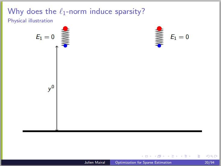
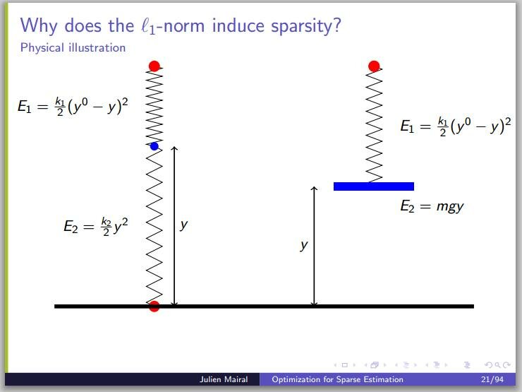
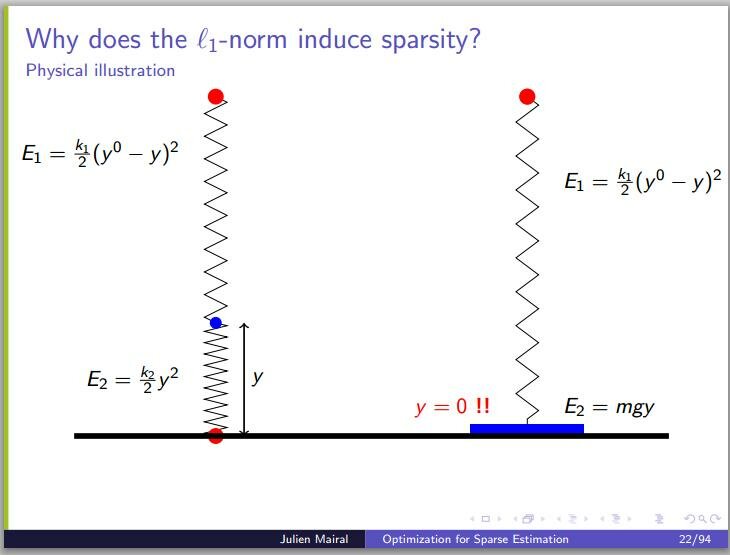
Perhaps a bit surprisingly, for the case of $L_1$ penalty (LASSO), one often gets solutions where some $|\beta_i|$ are not just small, but exactly zero. I recently came across an intuitive explanation of this fact based on a mechanical analogy, on a blog devoted to compressed sensing and related topics. The following three slides reproduced from a presentation by Julien Mairal perhaps do not exactly constitute a “proof without words“, but are really helpful nevertheless. The $E_2$ terms in the figures represent the $L_2$ and $L_1$ versions of the penalty function as “spring” and “gravitational” energies, respectively. Increasing the spring constant $k_2$ makes $y$ smaller, but not zero. Increasing the gravity (or the mass), on the other hand, eventually makes $y$ zero.

In case you haven’t seen it before, here is a visual from the original LASSO paper by Tibshirani, comparing $L_1$ and $L_2$ penalties in a two-dimensional problem ( $\hat{\beta}$ denotes the solution of the ordinary least squares problem, without any constraint or penalty):

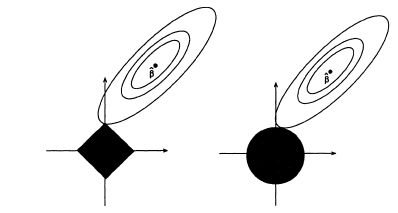
This provides another intuitive explanation of the sparsity of solutions obtained from LASSO. In order to make sense of this figure, you should keep in mind that the regularized problems above are equivalent to the constrained problem

$\text{Minimize } \sum_{i=1}^n (y_i - \mathbf{\beta}\cdot\mathbf{x}_i)^2\,,\\ \\\text{subject to } P(\mathbf{\beta})\le t\,,$

where $t\ge 0$ is analogous to the tuning parameter $\lambda$ , and $P(\mathbf{\beta})$ stands for $L_1$ or $L_2$ penalty, as above. (If this was a bit too cryptic, you can take look at the original LASSO paper, which, according to Google Scholar, has been cited more than 9000 times.)

L1 tidbits

Like this:

Leave a Reply Cancel reply

Recent Posts

Recent Comments

Archives

Categories

Meta

sitemeter